Signal Calculator
Signal Calculator lets you create new signals or instruments by combining existing SIGVIEW windows using arithmetic, mathematical, and signal-analysis functions.
Typical uses include:
•adding, subtracting, multiplying, or dividing signals and spectra;
•scaling or normalizing signals;
•combining signal values with instrument values or numeric constants;
•subtracting a signal mean or another calculated parameter;
•calculating cross-correlation and cross-spectral functions;
•performing convolution or custom smoothing;
•calculating Frequency Response Functions (FRF);
•performing Complex FFT and Inverse FFT operations;
•converting signals to and from the order domain [PRO].
Open Signal Calculator by selecting "System control/Signal calculator" from the main menu or by pressing the corresponding toolbar button:  .
.
Quick start
A calculator expression is created by combining existing windows with operators or functions.
For example, to subtract Signal B from Signal A:
Signal A - Signal B
1.Add Signal A to the expression.
2.Click the "-" operator.
3.Add Signal B.
4.Click OK.
SIGVIEW creates a new result window. The result remains linked to the source windows and is recalculated automatically whenever they change.
Creating an expression
The expression field at the top of the dialog shows the expression currently being created.
The left side of the dialog lists available signal and instrument windows from the current workspace. This includes loaded signals, acquisition signals, analysis results, calculated signals, and instruments.
You can filter the list to show:
•all windows;
•instruments only;
•signal-like windows only.
To add a window to the expression, either:
•double-click its name;
•select it and click ">>"; or
•click the corresponding window in the graphical workspace display below the list.
The graphical display works similarly to the Control Window. If a window cannot be used at the current position in the expression, it cannot be selected.
The right side of the dialog contains the available operators and functions. Only functions that are valid at the current position in the expression are enabled.
Window names in expressions
Windows with automatically generated titles are represented by their numeric identifier, for example: 17#
Windows with a custom title are represented by that title.
Giving frequently used windows meaningful custom titles can make longer calculator expressions easier to understand. Window titles can be changed from the corresponding window context menu or main-menu command.
Result windows and automatic updates
After completing the expression, click OK.
SIGVIEW creates a new signal or instrument window containing the result. The new window is linked to all source windows used in the expression and is recalculated whenever one of them changes.
If one of the source windows is deleted, the calculator result becomes frozen and retains its last calculated values.
For simple arithmetic operators (+, -, *, /), signal and instrument windows can be mixed in the same expression. If an expression contains only instruments and constants, the result is also an instrument window.
Combining signals of different lengths
If two signals with different lengths are used in a binary operation, SIGVIEW uses only as many samples as are available in the shorter signal.
For the longer signal, processing starts at its first visible sample.
When performing operations between two measured signals, make sure that the signals also represent compatible data, for example that their sampling rates, time alignment, and physical units are appropriate for the intended calculation.
Expression order and parentheses
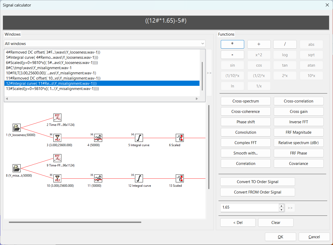
Signal Calculator builds expressions step by step and automatically inserts parentheses to make the calculation order explicit.
For example, if you first add A and B, then multiply the result by C, SIGVIEW displays the expression as:
(A + B) * C
If you continue by adding D, the expression becomes:
((A + B) * C) + D
This means that the calculation order is always mathematically unambiguous in the displayed expression.
The grouping is determined by the order in which the expression is created. Parentheses are generated automatically by SIGVIEW and cannot be inserted, removed, or rearranged manually. To obtain a different calculation order, build the expression in the corresponding sequence.
Numeric constants or instrument values
Numeric constants can be inserted by using the numeric field in the function area.

Constants can be used in positions where an instrument value can be used.
Examples:
Signal * 1000
multiplies every signal value by 1000.
Signal - 2.5
subtracts 2.5 from every signal value.
RMS_A / RMS_B
creates an instrument containing the ratio of two instrument values.
Available functions
Mathematical functions
The following unary functions can be applied to a signal or instrument:
•sqrt Square root
•log10 Base-10 logarithm
•ln Natural logarithm
•x^2 Square
•abs Absolute value
•2* Multiply by 2
•10* Multiply by 10
•(1/2)* Divide by 2
•(1/10)* Divide by 10
•1/x Reciprocal
•sin Sine
•cos Cosine
•tan Tangent
•atan Arc tangent
For signal windows, the selected function is applied to every signal value.
Arithmetic operators
The following binary arithmetic operators are available:
•* Multiply
•/ Divide
•+ Add
•- Subtract
They can be used with signals, instruments, and numeric constants where applicable.
Signal operations
Cross-correlation: Calculates the cross-correlation between two signals as a function of their relative time shift. See [link: Cross-spectral analysis].
Convolution: Convolves the first signal with the second signal. Convolution is commonly used to model the response of a linear system, apply an impulse response, or perform custom filtering.
Smooth with: Smooths the first signal by using the second signal as a custom weighting function (kernel). This allows user-defined smoothing beyond the standard built-in smoothing functions.
Cross-spectral and frequency-response functions
The following functions operate on two signals in the frequency domain:
See Cross-spectral analysis and Frequency Response Function (FRF) for details.
Complex FFT functions
Complex FFT: Calculates the FFT of a complex-valued signal represented by separate real and imaginary signal components.
Inverse FFT: Converts a complex spectrum, supplied as separate real and imaginary components, back to the time domain.
See Inverse FFT for details.
Order Analysis functions [PRO]
The following Order Analysis functions are available in SIGVIEW PRO:
- Convert TO Order Signal
- Convert FROM Order Signal
Editing the expression
Clear: Removes the complete expression.
< Delete: Removes the last entry from the expression.
Examples
Below are some examples of calculator expressions:
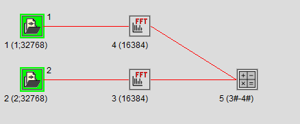
1. Simple arithmetic operations on spectra
You have loaded two signals, calculated their spectra and you have the following workspace:
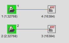
Now, you would like to subtract two calculated spectra to get some information about their differences. To do so, create the following expression in the Signal calculator:
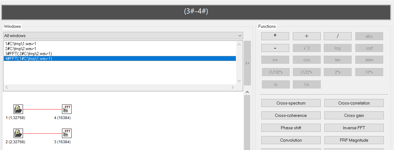
The resulting window will contain the requested difference between spectra.
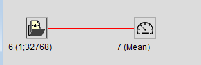
2. Combining instruments and signals in one expression.
You would like to subtract the mean value of a signal from all signal values (normalisation). Firstly, you would calculate signal mean by using the appropriate instrument:
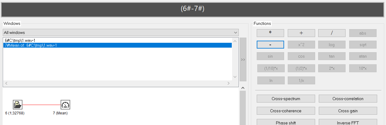
Then, you would create the following expression in the Signal calculator:
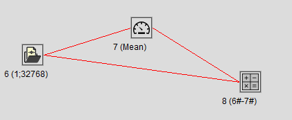
The result will be a new signal calculated as requested:
2. Instrument-only expressions
You can also create expressions containing only instrument windows. The result of such expressions will also be a new instrument window.
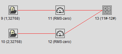
In this example, we calculate the RMS of two signals and then create a new instrument containing their difference:
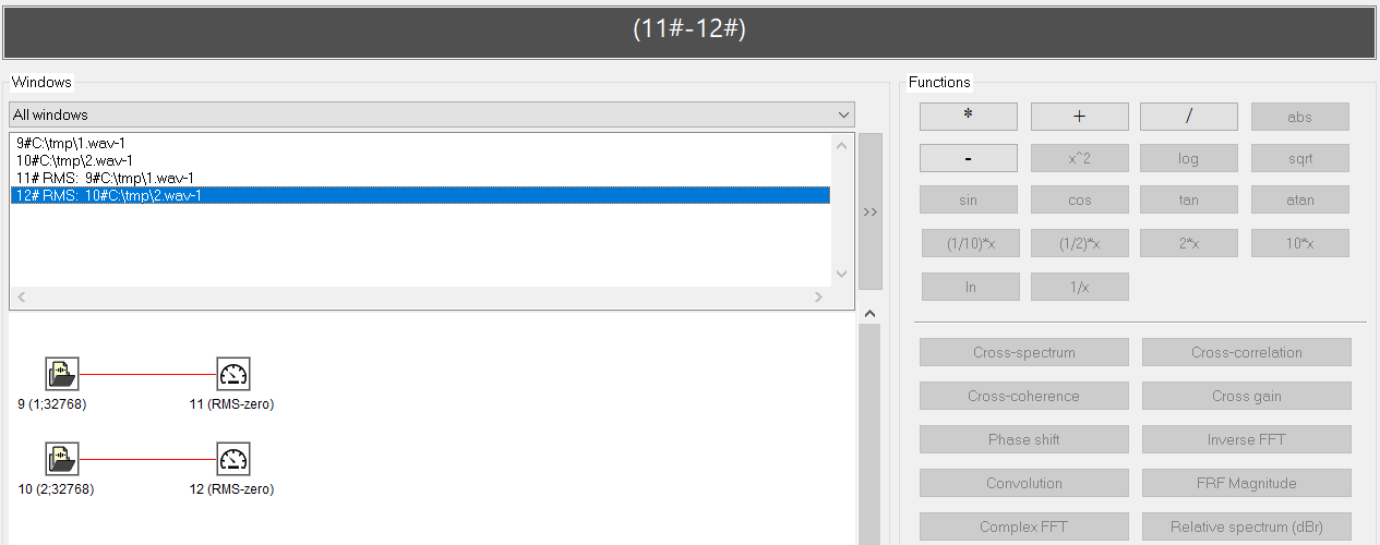
The result will be a new instrument window:
3. Complex expressions.
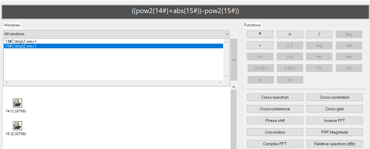
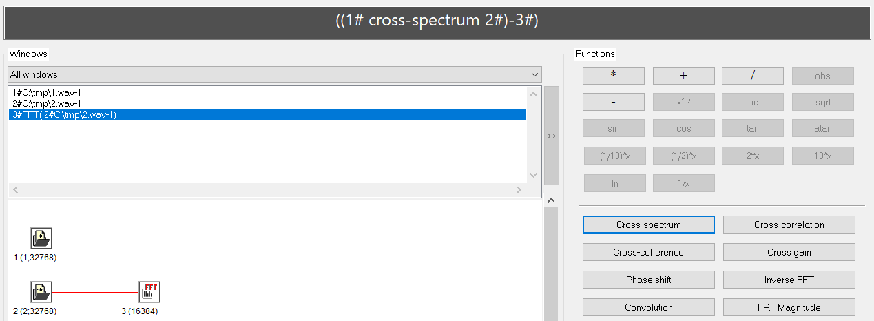
There are practically no limitations for creating calculator expressions. Here are some examples:
f = A^2 + abs(B) - B^2
Subtract spectrum of one signal from its cross spectrum with another signal
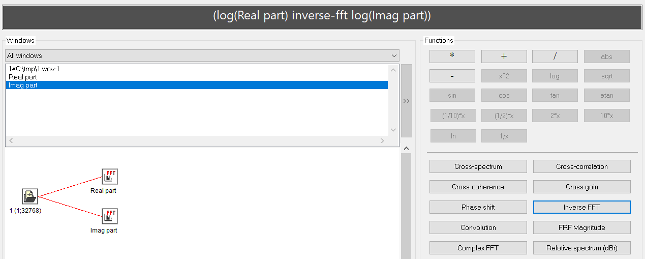
Calculate log-values of both real and image spectrum and then perform inverse FFT