Spectral Analysis Defaults
Most spectral analysis tools in SIGVIEW are based on the FFT algorithm. There are many different parameters which can be applied to the signal before the FFT analysis is performed, to the FFT calculation itself, or its result.
If you want to change the default settings for spectral analysis calculation in SIGVIEW, use the “Signal tools/Spectral analysis” default option from the main menu. These settings will be applied to all new FFT-based calculations, including FFT, Time-FFT, cross spectral analysis, etc.
Once the FFT or Time-FFT has already been calculated according to your current spectral analysis defaults, you can edit those anytime by selecting the “Edit/Properties” menu option for the calculated window (FFT, Time-FFT…). The same option is also available in the window’s context menu. These settings will apply only to that single window.
The following parameters can be changed for each FFT based spectral analysis operation in SIGVIEW:
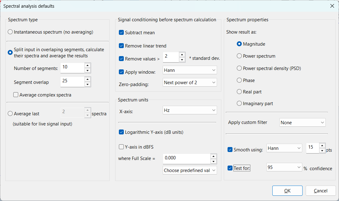
Spectrum type
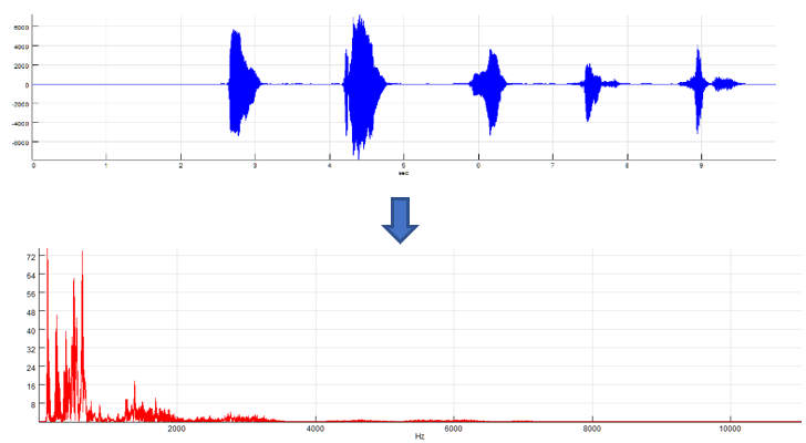
•Instantaneous spectrum (no averaging): Each change in the signal will cause the spectrum to be calculated again. A single spectrum will be calculated from the complete visible signal part of the source window. This is the default behaviour.
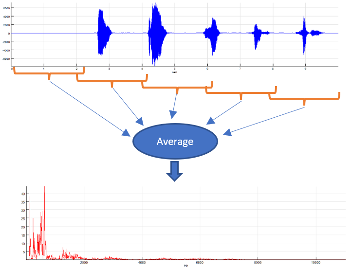
•Split input in overlapping segments, calculate their spectra and average the results: By using this method, the input signal will be split in overlapping segments based on the user-defined settings (number of segments and the overlap percentage). A separate (complex) spectrum is calculated from each of segments, the resulting spectra are averaged, and the result is displayed. By using 'Average complex spectra' checkbox, you can determine if the averaging will be applied to the complex result of the FFT algorithm (complex averaging) or to the final result of the calculation (e.g. magnitude, power, PSD...). If applied to PSD values, this method is also known as "Welch's Method" for the PSD calculation. The averaging will decrease the influence of the noise in the signal. This averaging method is suitable for live and offline signals, because it does not need consecutive updates of the input signal in order to calculate the average. But, splitting input signal in segments will also reduce the spectral resolution.
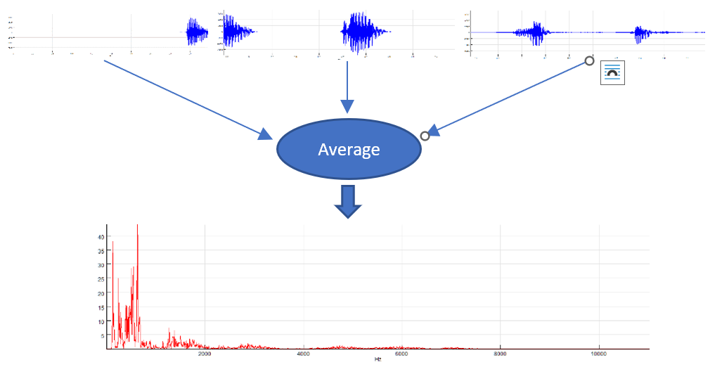
•Average last X spectra: This option is useful only for the FFT of the live input signal or other fast changing signals. On each change of the input signal (for example, a new data block from DAQ device), new spectrum will be calculated and stored in the averaging buffer. After X spectra are calculated for X data blocks, those will be averaged to calculate the resulting spectrum, which will be displayed. The averaging will decrease the influence of the noise in the signal. Since at least X updates in the input signal are needed to calculate one spectra, this method is suitable only for live signals (DAQ signals or moving smaller signal parts through the whole signal). If you try to use it on a loaded signal file, it will do nothing, because it will wait for subsequent updates of the signal to be able to calculate the average.
Signal conditioning before spectrum calculation
Subtract mean check box: Select this if you want to normalise the signal before processing. It simply subtracts the mean value of the signal from each sample.
Remove linear trend check box: If linear trend appears in signal (i.e. the whole signal rises or falls monotonously), it can affect the evaluation of low frequency components in the FFT. This option removes linear trend by subtracting linear least squares approximation from the signal.
Remove values >: This option automatically removes values from the signal that are not in range (mean - N*StDev, mean + N*StDev) where StDev is a standard deviation of the signal and N is a user-defined coefficient entered in the corresponding edit box. Values are removed by replacing them with the mean value.
Apply window: To avoid some undesirable effects of discrete Fourier transform (DFT), it is recommended to lower the signal values near the end of the signal by multiplying it with some appropriate weighting function. This technique is called “windowing”. SIGVIEW supports several standard weight functions: Hann, Hamming, Blackman, Triangle, Tukey, Kaiser, Flat top, Blackman-Harris, Nuttall, Gaussian, Exponential. Selecting the “Rectangle” window has the same effect as turning the windowing option off.
Exponential window is the only one which is not symmetrical. It is usually used for impact testing signals where signal begin (impulse) is more important than the rest of the signal.
Zero padding: Due to the nature of the FFT algorithm, the fastest calculation will be performed for signals having a power-of-2 length (for example 128, 256, 512…). If your signal or the part you would like to analyse has some other length, there are several options you can choose:
oNever use zero padding: FFT or a slower DFT algorithm will be applied on your signal without altering or extending it with zeros. This is the slowest calculation method, but the advantage is that your signal is not changed in any way. For prime number signal lengths, the calculation will be performed by using a very slow DFT algorithm
oOptimal method: Your signal will be expanded with zeros to the next possible length, allowing the usage of the FFT algorithm instead of a very slow DFT
oNext power-of-2: Your signal will be expanded with zeros until the next power-of-2 length. This will enable the usage of the fastest FFT algorithm
To increase the precision of the spectral analysis without taking longer signal segments, you can also expand the existing signal segment with zeros, even beyond the next power-of-2 length. That will not add essentially new information to the FFT result, but will increase its precision; i.e. will reduce the size of the one frequency bin. You will simply get an FFT result with more points, from the same signal segment. (If the signal has 1024 samples and you choose expanding by factor 8, the resulting spectrum will have 4096 pt. instead of 512, without using this option). The result will be comparable to interpolation of the normal FFT result. To use this feature, you can choose the 2x, 4x or 8x zero padding options.
Spectrum units
Logarithmic Y-Axis (dB units): This option can only be applied to Magnitude, Power spectrum and PSD spectrum results. It shows the logarithmic values for all FFT result points, causing the Y-axis to be logarithmic.
Y-axis in dBFS: This option can only be applied if the logarithmic Y-Axis is used. It will calculate dB values relative to some maximal, i.e. full scale value. You can freely define this full-scale value in signal units (for example, 32767 for 16-bit sound card or max. voltage for NiDAQ devices). There is also a combo-box with the choice of some predefined values for the maximal amplitude. If you set the full scale value to 0 dB, values will always be calculated relative to the currently highest FFT value; so that the highest value is always equal to 0 dB and all other FFT values are negative.
X-Axis unit combo box: This allows you to switch between the following X-axis units: “Hz (Cycles/sec)”, “CPM (Cycles/minute)”, “KHz”, “MHz”.
Spectrum properties
Show result as: After applying the FFT algorithm to the signal, the result will be an array of complex numbers. These radio-buttons determine the method which will be used for converting complex numbers to real values in order to display them in a resulting graphic.
oMagnitude: Often generally regarded as “spectrum”; calculated as sqrt(R^2 + I^2)
oPower spectrum: Magnitude squared
oPower spectral density (PSD): Power spectrum is calculated first and its values are divided with the width of the frequency bin. This “normalisation” makes comparisons between FFT sequences from different signals with different sampling rates possible
oPhase: Show signal phase angle (in degrees)
oReal & Imaginary part: Show only real or only imaginary part of the spectrum
Apply custom filter curve: You can apply a custom filter curve to change the values of the spectrum. See the Custom filter curves section for more information. This option is applicable only to magnitude and power spectrum result types.
Smoothing: If the FFT result is noisy and has many values, it can be useful to smooth it by using the weighted moving average function. That will remove small noisy details from the FFT and give you a better overview of the important spectrum events. You can choose some standard weighting functions here and determine the length of a smoothing window (longer window means more smoothing).
Test for confidence: Siegel’s test for confidence of spectral peaks tells you if some peak in the spectrum is statistically significant or it could be a product of some random fluctuation of the signal. If you turn this option on, only significant peaks will be shown, while all other values in the spectrum will be set to zero. You can choose two levels of confidence for this test: 95% or 99%. This test is purely statistical; it does not use any artificial intelligence methods.
Fast access to predefined spectral analysis settings
All FFT-based functions (FFT, Time-FFT, Spectrogram) offer a fast access to some commonly used spectrum variants directly in toolbar. These variants are stored as Tool windows (*.swt) in the "FFTVariants" subfolder of the SIGVIEW Application Data folder. By saving new FFT-based tools in that folder, you can add new variants which will appear automatically in the toolbar, next to the standard installed variants.
