
Octave Plots
Octave band analysis is a method of analyzing the frequency content of a signal by dividing the frequency range into bands that are proportional in width. In a standard full-octave plot, each band spans a frequency range that is twice the width of the previous one and half the width of the next. This type of analysis is particularly suited for acoustic and audio measurements, as it aligns with how the human ear naturally perceives sound.
By grouping frequencies into octave bands, it's easier to compare sound energy levels across a broad range, offering meaningful insights into the subjective quality of sound - such as loudness or tonal balance.
Fractional Octave Plots
To achieve greater frequency resolution, octave bands can be subdivided into smaller intervals:
•1/3 Octave
•1/6 Octave
•1/9 Octave
•1/12 Octave
These options are available in SIGVIEW as separate functions and follow the same principle as standard octave analysis but offer finer frequency granularity, making them ideal for detailed sound measurement and analysis.
All octave plot functions can be accessed via the “Signal Tools” menu:

Implementation
In SIGVIEW, octave analysis is implemented using a Custom Filter bank plot, rather than FFT-based methods. This approach ensures compliance with established acoustic measurement standards, such as ISO 266, which define the behavior and structure of octave bands.
Each octave type uses a corresponding filter bank definition file located in the "filters" subdirectory of the SIGVIEW application data directory. The files are named "octave filter.flb", "1_3_octave_filter.flb", "1_6_octave_filter.flb" etc.
These files contain the frequency definitions for each filter bank and can be freely edited using a text editor to customize the analysis to your specific needs. For details on how to modify filter banks, refer to the custom filter bank chapter.
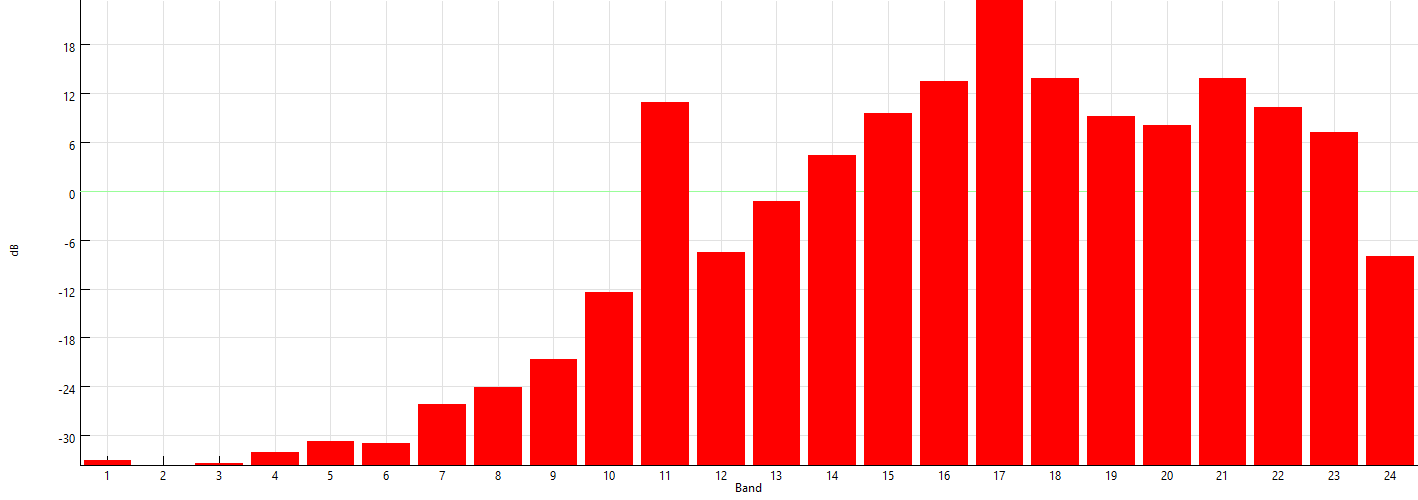
By default, octave plots are displayed by using the histogram display type (min-reference). As for all other plots, you can change the display type by using a context menu or toolbar buttons (Signal Display options).
Frequency markers:
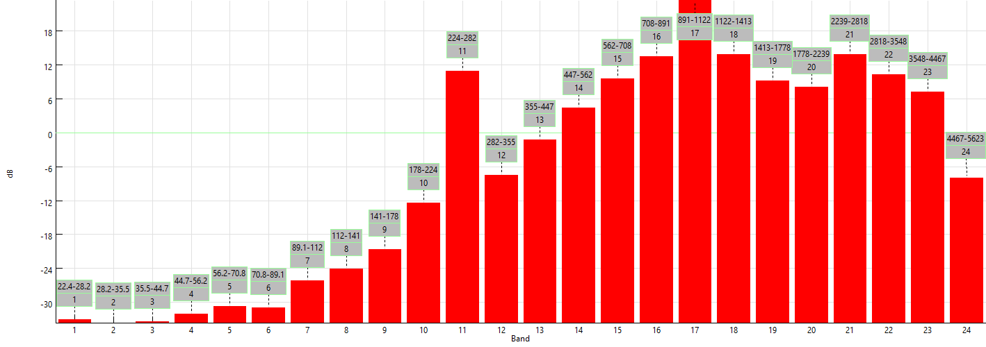
By default, the X-axis shows only band numbers. To see each band's frequency range instead, enable "Show frequency markers" from the plot's context menu — this displays a marker above every band showing the frequency range used to calculate its value. To make this the default for all new octave and custom filter plots, enable the corresponding option on the Display tab of Application settings.
Switch between linear/dB values display:
By default, octave and custom filter plots show values in dB units. To view them in signal's linear units instead, disable "Show values in dB" from the plot's context menu — this converts the Y-axis to a dB scale and updates the axis label accordingly.
Histogram bar spacing:
The spacing between bars in histogram-style plots can be adjusted using the "Space between histogram bars" option on the Display tab of Application settings.
Applying A-weighting or C-weighting to an Octave Plot
Octave and custom filter bank plots can display band levels with A-weighting or C-weighting applied, so the displayed levels better reflect how the human ear perceives loudness at different frequencies — the same weighting curves used in sound level meters.
Why weight the bands at all?
The human ear is not equally sensitive to all frequencies: at typical listening levels it's markedly less sensitive to very low and very high frequencies than to the 1–4 kHz range. A raw (unweighted) octave-band level in dB treats every band the same, which is exactly what you want for pure signal analysis — but it can be misleading if what you actually care about is how loud something sounds, or if you need results that are comparable to a sound level meter reading in dB(A) or dB(C).
A-weighting closely follows the ear's sensitivity curve at normal listening levels. It attenuates low frequencies strongly and high frequencies moderately, leaving the mid band (around 1–4 kHz) essentially unchanged. It's the standard weighting for environmental and occupational noise measurements (dB(A)).
C-weighting is much flatter across the audible range, with only mild roll-off at the extreme low and high ends. It's commonly used for peak/impulse noise measurements and for evaluating low-frequency content that A-weighting would otherwise mask.
How to enable it
1.Create an Octave plot (or a Custom filter bank plot) from any signal window.
2.Right-click anywhere in the plot to open the context menu.
3.Choose Apply A-weighting or Apply C-weighting. The chosen option is applied immediately and is shown with a checkmark; choosing it again (or switching to the other weighting) turns it off.
Weighting can be combined with the existing Show values in dB option, or used with linear values — the weighting gain is applied to each band's level before any dB conversion.
Only one weighting can be active at a time (A, C, or none) — selecting one automatically deselects the other.
Notes
Weighting is applied per band, using each band's own center frequency — the same standard A/C-weighting curves already used elsewhere in SIGVIEW (e.g. for FFT custom filters).
The selected weighting is saved with the window and restored when the workspace is reloaded, just like the dB/linear display setting.
This applies to both standard octave plots (1/1, 1/3, 1/6, 1/9, 1/12) and custom filter bank plots created from a .flb file.