Custom Filter Curves
What is a custom filter curve?
SIGVIEW allows you to define custom filter curves and to apply those during time-domain signal filter or for spectrum modification. The custom filter curve is actually a sequence of [frequency, modification factor] pairs which define how a frequency component should be changed.
For example, a band-pass filter with a pass-band between 1000 - 2000Hz could be defined this way:
1000 0.0
2000 1.0
20000 0.0
Meaning that all frequency components up to 1000Hz should be removed (factor 0.0), all frequencies between 1000Hz and 2000Hz should remain intact (factor 1.0) and all frequencies above 2000Hz up to 20000Hz should be removed (factor 0.0).
Another example would be a standard a-weighting curve used in sound pressure level measurement. This curve is defined in dB, i.e. signal increase, or decrease dB level for certain frequencies:
10 -70.43
20 -50.39
30 -40.6
40 -34.54
50 -30.27
Meaning that frequency components around 10Hz should be reduced for -70.43dB, around 20Hz for -50.39 dB and so on. Note that we do not define upper frequency limits here as in the first examples but centre the frequencies of each "bin".
What is included in SIGVIEW?
SIGVIEW allows you to define all those filter types manually (by editing text files) or from existing spectrum curves and to apply them to signals or spectra. All filter curves used by SIGVIEW are stored in a "filters" subdirectory of the SIGVIEW data directory (usually C:\Documents and Settings\<UserName>\Application Data\Sigview\). For more information about filter file structure and creation, see below.
The following filter curve types are supported:
Magnitude values filter: Filter values are used as absolute magnitude values in signal units. The filter amplitude values will be subtracted from the actual signal values when the filter is applied (magnitude reduction). This means that a value of 5 in a filter for certain frequency will actually reduce signal amplitude on that frequency for 5 signal units (for example, Volts) when the filter is applied. This filter will mostly be created from existing spectrum curves. For example, you can use SIGVIEW to calculate your microphone characteristic response curve, save it as a filter, and subtract from a spectrum of the recorded audio.
Relative dB values filter: As in the second example above, this filter contains dB values to modify certain frequency components. For example, a value of -50 means that the frequency component will be reduced for 50dB.
Relative values filter: As described in the first example above, this filter contains relative coefficients which are used to multiply frequency components on certain frequencies (for example, 0.5 means that the frequency component is reduced to 50%). This type of filter will mostly be created manually by editing the filter file with editor.
Creating custom filter curves manually
Custom filter curves are stored in plain-text files with the extension *.flt, and stored in a "filters" subdirectory of the SIGVIEW installation directory. You can create these files in any text editor and save them into the "filters" directory located in SIGVIEW's application data directory (usually C:\Documents and Settings\<UserName>\Application Data\Sigview\). At the next start-up, SIGVIEW will read your file and include it in all filter functions. Each filter has 3 header lines at the beginning, looking similar to these:
Type=DB_ADD
Frequency=CENTER
########
10 -70.43
20 -50.39
30 -40.6
These lines are followed by rows containing frequency in Hz/value pairs using TAB (ASCII 0x9) as a value separator. For an example, please take a look at delivered "a-weighting.flt" file.
Type parameter (Type=) in the FLT file defines which type of filter is in the file.
The following values are allowed:
ABS_SUB: Corresponds to the "Magnitude values filter" as described above. Following filter values will be interpreted as magnitude values and subtracted from corresponding signal magnitude values.
DB_ADD: Corresponds to the "Relative dB values filter" as described above. Following filter values will be interpreted as dB values defining how to modify a certain frequency component (for example, -50 means that signal magnitude on that frequency will be reduced by 50dB).
ABS_MUL: Corresponds to the "Relative values filter" as described above. Following filter values will be interpreted as coefficients to multiply a certain frequency component with (0.5 means reduction of the magnitude for 50%).
The frequency parameter defines how to interpret frequency values.
The following values for this parameter are allowed:
CENTER: Frequency value is centre frequency. Corresponding filter value will be applied to all frequencies ( (fi + fi-1)/2, (fi+fi+1)/2 ].
MAX: Frequency value is an upper limit frequency. Corresponding filter value will be applied to all frequencies ( fi-1, fi].
Creating custom filter curves in SIGVIEW
You can save any signal or analysis result from SIGVIEW as a filter curve. You will usually start with a magnitude spectrum or its averaged version. It can be directly saved as a "Magnitude values filter". The ratio between two spectra can, for example, be stored as a "Relative values filter". In all cases, you will use the “File/Save as filter curve...” main menu option on a window containing your filter sequence. The following dialog appears after opening this menu item:
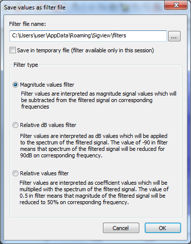
You have to define the file name of your filter. It has to have an FLT extension and it should be stored in the "filters" directory under SIGVIEW's application data directory (usually C:\Documents and Settings\<UserName>\Application Data\Sigview\). Otherwise, it will not be visible to SIGVIEW. You can also decide to store the filter as a temporary file. In that case, you should only give it a name - there will be no file actually stored on disk. Of course, the filter will be lost when you close SIGVIEW. In the “Filter type” box you have to tell SIGVIEW what type of filter it is, i.e. how to interpret filter values later when applying the filter. These types correspond exactly to the filter types explained above. After you press OK, the filter will be saved and will be accessible from the filter and spectrum properties functions.
All filters stored in this way will use the CENTER setting to interpret frequency values (see above).
To delete a filter, simply delete its *.FLT file in the filters directory.
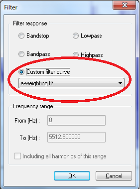
Using custom filter curves for time-domain signal filtering
You can use custom filters to directly filter time-domain data. This feature is implemented as a part of the “Signal tools/Filter...” menu option. After applying your filter to a time-domain signal, the difference, (or ratio) between magnitude spectrum of the original signal and magnitude spectrum of the filtered signal will correspond to the custom filter curve.
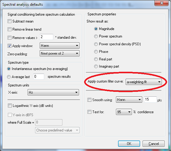
Using custom filter curves for spectrum modification
You can use custom filters to modify calculated magnitude spectrum or power spectrum just as if the filter were applied to the origin time-domain data. This option is available from the Properties dialog of any spectrum window or as a general setting in the Spectrum Analysis defaults dialog. After applying your filter to a spectrum, the difference, (or ratio) between original spectrum and modified spectrum will correspond to the custom filter curve.
No matter what the type of your custom filter is (dB, absolute...), SIGVIEW will be able to apply it to all spectrum types; i.e. a dB filter will also be applicable on magnitude spectrum with linear scale values. SIGVIEW will perform all needed filter conversions internally.
For more information, see the ‘Use custom filter curve for better measurement results’ section.